Estimation#

This page estimates the model parameters. We will do this in two steps:

Using a grid of parameters values
Using a Optimizer

Warning

Remember that dhr.func is the sintax that calls the file with the functions see before.

Packages#

import time
import numpy as np
import pandas as pd
import seaborn as sns
import dhr_functions as dhr
from scipy.optimize import minimize
from matplotlib import pyplot as plt

Calling the simulated data for the treatment#

First we will call our simulated data using the function and transform in a dictionary. The dictionary makes the estimation faster. The dataframe_simulation function creates two dataset (control and treatment) and put them in a dictionary to return. dataset is going to store this dictionary.

dataset = dhr.dataframe_simulation()
dataset['treatment']

	id	t	d+1	d	L	eps	U
0	0	1	1.0	0.0	0.0	-0.572858	50.736634
1	0	2	2.0	1.0	0.0	0.154607	50.538425
2	0	3	2.0	2.0	1.0	1.889621	51.730462
3	0	4	3.0	2.0	0.0	-0.613751	48.642785
4	0	5	4.0	3.0	0.0	-0.192819	48.444930
...	...	...	...	...	...	...	...
2995	99	26	18.0	17.0	0.0	0.194402	33.791186
2996	99	27	19.0	18.0	0.0	-1.103202	33.593390
2997	99	28	20.0	19.0	0.0	-0.675562	33.395593
2998	99	29	21.0	20.0	0.0	-1.585189	33.197797
2999	99	30	22.0	21.0	0.0	0.482229	1100.000000

3000 rows × 7 columns

Select the group you want and take it from the dictionary. We will use the treatment.

data = dataset['treatment'].to_dict('records')

Example with initial values#

Now, set the initial values for the estimation, the list is [beta, theta]. After determining this, call the model solution to extract the probabilities of working and leisure.

theta=[0.01,4.5]
probs_w, probs_l, _, _, _, _, = dhr.model_solution(beta = theta[0], mu = theta[1]);

Now we will calculate the Maximum Likelihood for a specific initial value. This will be repeated multiple times in the estimation in order to find the minimu log likelihood value.

logL = 0
for i in range(len(data)):
    t = int(data[i]['t'])
    d = int(data[i]['d'])
    L = int(data[i]['L'])
    likelihood = np.log(probs_w[t-1,d])*(1-L)+ np.log(probs_l[t-1,d])*L
    logL = logL + likelihood 

Now, check the value

-logL

4619.478266596326

Our estimation wants to minimize this, in order to match the model solution and the simulated data. Let’s see this in two ways:

Using a grid of parametes values
Optmizer

Grid of values#

We will create a grid of values for beta and mu. After that, we will compute the Likelihood of the combinations and pick the combination that generates the lowest value.

n = 10
b_guess  = np.linspace(0.01, 0.04,n)
mu_guess = np.linspace(3, 4.5,n)

Above I create a grid with 10 values each for beta and mu. Let’s compute the Likelihoods. I will use a function called Log_likelihood(), wich computes and stores parameters combinations and repective likelihood values in a dataframe.

start = time.perf_counter()
log_values = dhr.Log_likelihood(data, b_guess, mu_guess)
maxL = log_values['likelihood'].max()
optb = round(log_values.loc[ log_values['likelihood'] == maxL]['beta'].item(),2)
optmu = round(log_values.loc[ log_values['likelihood'] == maxL]['mu'].item(),2)
end = time.perf_counter()

Let’s see the result

print('optimun beta:' + str(optb) +'\noptimun mu:' + str(optmu))
print("Elapsed (with compilation) = {}s".format((end - start)))

optimun beta:0.03
optimun mu:4.0
Elapsed (with compilation) = 10.396148917000001s

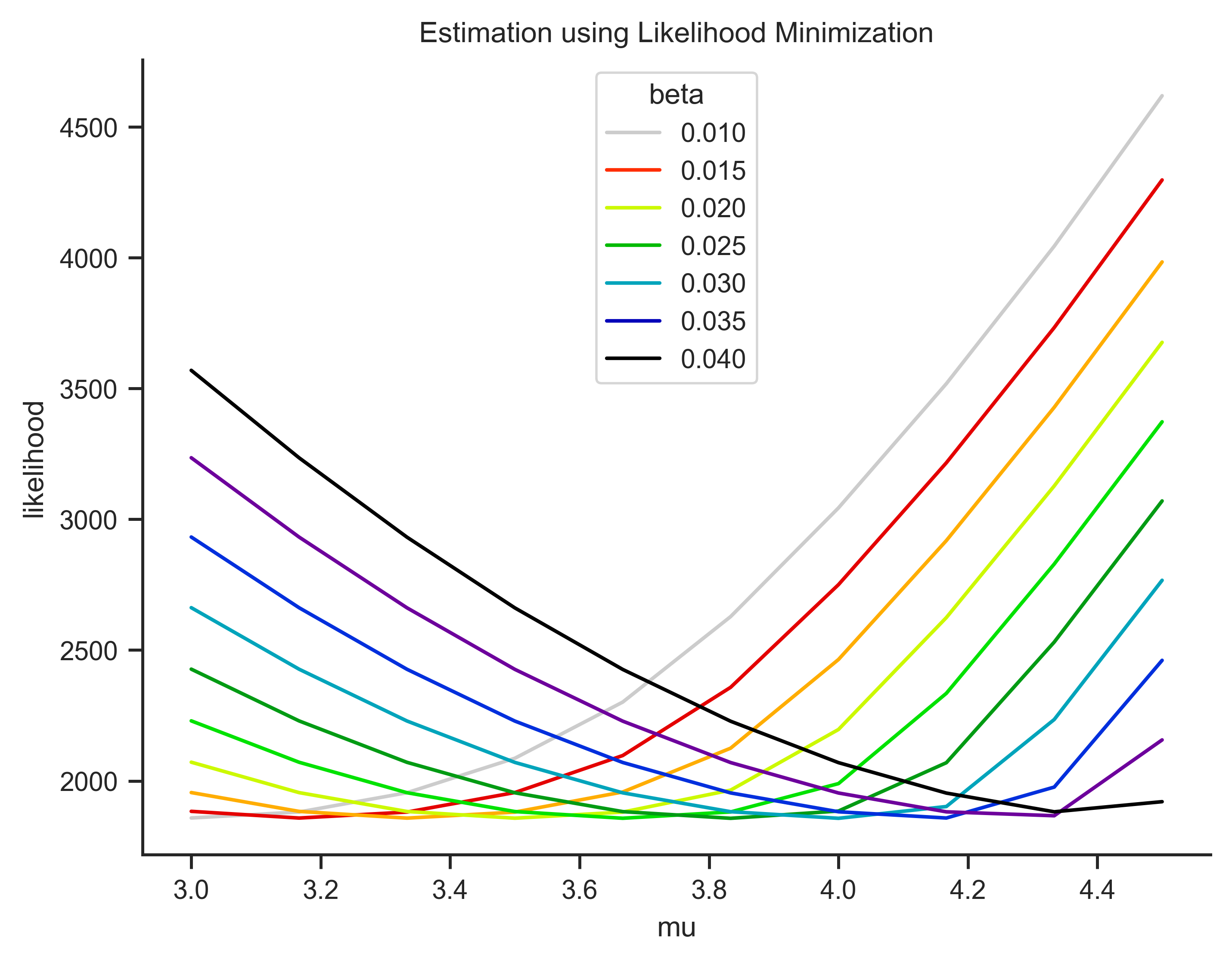
The result is exaclty the parameters estimated in the model. Now, lets plot this and see graphically.

# PLOTTING SETTINGS
plt.rcParams['figure.dpi'] = 500
plt.rcParams['savefig.dpi'] = 500
sns.set_style('ticks')
sns.despine(left=False, bottom=True)
sns.set_context("paper")

<Figure size 3200x2400 with 0 Axes>

Above I just defined settings to improve plotting quality

sns.lineplot(data = log_values, x = 'mu', y = (log_values['likelihood']*-1), hue = 'beta', palette= 'nipy_spectral_r' ).set(title = 'Estimation using Likelihood Minimization')    
sns.despine(left=False, bottom=False)

Optimizer#

Now, use a minimizer (here minimize from scipy package) to find the parameters values that minimizes the log likelihood. We need to define the function used to estimate the logLikelihood and put this as an argument of the function (opt_likelihood). Also, we need to choose the initial guess and method.

def opt_likelihood(theta):
    probs_w, probs_l, _, _, _, _, = dhr.model_solution(beta = theta[0], mu = theta[1]);
    logL = 0
    for i in range(len(data)):
        t = int(data[i]['t'])
        d = int(data[i]['d'])
        L = int(data[i]['L'])
        likelihood = np.log(probs_w[t-1,d])*(1-L)+ np.log(probs_l[t-1,d])*L
        logL = logL + likelihood 
    return -logL

start = time.perf_counter()
resu = minimize(opt_likelihood, theta, method = "SLSQP" )
end = time.perf_counter()

/Users/angelosantos/Documents/GitHub/human-capital/websites/hc_routines/myst/dhr/dhr_functions.py:151: RuntimeWarning: invalid value encountered in double_scalars
  e_exp = eps_mean + (eps_sd*norm.pdf((eps_thres-eps_mean)/eps_sd)/(1-norm.cdf((eps_thres-eps_mean)/eps_sd)));
/var/folders/sb/z5dkqpwn7pzchsbq06rbbm9w0000gn/T/ipykernel_16298/2744515528.py:8: RuntimeWarning: divide by zero encountered in log
  likelihood = np.log(probs_w[t-1,d])*(1-L)+ np.log(probs_l[t-1,d])*L
/var/folders/sb/z5dkqpwn7pzchsbq06rbbm9w0000gn/T/ipykernel_16298/2744515528.py:8: RuntimeWarning: invalid value encountered in double_scalars
  likelihood = np.log(probs_w[t-1,d])*(1-L)+ np.log(probs_l[t-1,d])*L
/Users/angelosantos/Documents/GitHub/human-capital/websites/hc_routines/myst/dhr/dhr_functions.py:151: RuntimeWarning: divide by zero encountered in double_scalars
  e_exp = eps_mean + (eps_sd*norm.pdf((eps_thres-eps_mean)/eps_sd)/(1-norm.cdf((eps_thres-eps_mean)/eps_sd)));
/Users/angelosantos/Documents/GitHub/human-capital/websites/hc_routines/myst/dhr/dhr_functions.py:237: RuntimeWarning: invalid value encountered in double_scalars
  vf[t-1,d] = probs_l[t-1,d]*(VF(L = 1, t = t, d = d, beta = beta, mu = mu,  g=g, I = I, M = M, eve_l = eve_l[t-1,d])) \

Now, print the results and see that the values that minimize the function are close to beta = 0.03 and mu = 4, the estimated values from the paper.

print('Optimun beta:' + str(round(resu.x[0],2)) + "\n" + 'Optimun mu:' + str(round(resu.x[1],2)))
print("Elapsed (with compilation) = {}s".format((end - start)))

Optimun beta:0.03
Optimun mu:3.93
Elapsed (with compilation) = 5.028053667s

Human Capital

Estimation

Contents

Estimation#

Packages#

Calling the simulated data for the treatment#

Example with initial values#

Grid of values#

Optimizer#