Simulation
Contents
Simulation#
Packages#
import numpy as np
import pandas as pd
import ams_functions as ams
Using the Model solution#
Using the model solution we can get the expected value matrix to use in our simulation. We will use this to calculate the utility for working and going to school.
probs_w, probs_s, eps_t, eve_w, eve_s, vf = ams.solution()
Simulation#
Parameters#
We need to define how many individuals we are going to simulate and other parameters for our simulation. The parameters are:
Shock mean (
ϵ_mean)Shock Standart deviation (
ϵ_sd)The age that we start simulating children choices (
age_start)The maximum additional years to
age_start. In our case we willage_start+age_max= 15, 15 is the last year that we are going to simulate.Number of individual (
sim)Discount factor (
β)
About the shock, we are considering a logistic distribution.
np.random.seed(1996)
ϵ_mean    = 0
ϵ_sd      = 1
age_start = 6
age_max   = 10
sim       = 100
β         = 0.9
Creating Matrices#
Now, we need to create the matrices to store our results and create a dataframe with our individual. We will store the following:
Schooling decision
Education Level in the current period
Education Level in the next period
Age of the child
Shock received
Utility obtained from decision
Consumption obtained from decision
# School decision
S_dec = np.empty((age_max,sim))
S_dec[:] = np.nan

# Education level (current period)
ed_cur = np.empty((age_max,sim))
ed_cur[:] = np.nan

# Education level (next period)
ed_next = np.empty((age_max,sim))
ed_next[:] = np.nan

# Age
age_c = np.empty((age_max,sim))
age_c[:] = np.nan

# Shock
eps = np.empty((age_max,sim))
eps[:] = np.nan

# Utility
U = np.empty((age_max,sim))
U[:] = np.nan

# Comsumption
C = np.empty((age_max,sim))
C[:] = np.nan
Simulating the individuals#
Now we will loop our simulated individuals using the vf matrix obtained using the model solution code. The loop is commented in order to understand the steps.
# Loop to simulate the individuals
for s in range(sim):
    # All the individuals start with no education
    edu = 0
    for age in range(age_max):
        # Actual child's age
        age_c[age,s] = age_start + age
        ed_cur[age,s] = edu

        # Random shock to education cost
        e_shock = np.random.logistic(loc = ϵ_mean, scale = ϵ_sd)

        # Random shock to primary education sucess
        e_sucess = np.random.uniform()

        if age == age_max - 1:
            s_ev = ams.prob_progress(edu)*ams.terminal_v(edu=edu+1) + (1 - ams.prob_progress(edu))*ams.terminal_v(edu=edu)
            w_ev = ams.terminal_v(edu=edu)
        else:
            s_ev = ams.prob_progress(edu)*vf[age+1, edu+1] + (1 - ams.prob_progress(edu))*vf[age+1,edu]
            w_ev = vf[age+1, edu]

        # Utility for choices
        school = ams.utility(age, edu, school=1, ϵ = e_shock) + β*s_ev
        work   = ams.utility(age, edu, school=0, ϵ = e_shock) + β*w_ev

        # Decision that max utility for individual
        dec = max(school, work)
        u = dec
        if u == school:
            if e_sucess <= ams.prob_progress(edu):
                suc = 1
            else:
                suc = 0
            ed_next[age,s] = edu + suc
            C[age,s] = ams.budget_constraint(age, edu, school=1)
            U[age,s] = dec
            S_dec[age,s] = 1
        else:
            suc = 0
            ed_next[age,s] = edu + suc
            C[age,s] = ams.budget_constraint(age, edu, school=0)
            U[age,s] = dec
            S_dec[age,s] = 0
        eps[age,s] = e_shock
        edu = edu + suc
Now we can use the data created to build our dataframe.
simulated_data = []
for i in range(sim):
    s = {}
    s['id'] = i
    s['age']  = list(range(6,16))
    s['edu']  = list(ed_cur[:,i])
    s['edu_next'] = list(ed_next[:,i])
    s['School']  = list(S_dec[:,i])
    s['eps']  = list(eps[:,i])
    s['U']  = list(U[:,i])
    s['C']  = list(C[:,i])
    s = pd.DataFrame(s)
    simulated_data.append(s)

simulated_data = pd.concat(simulated_data, axis = 0).reset_index().drop('index', axis = 1)
print(simulated_data)
     id  age  edu  edu_next  School       eps           U           C
0     0    6  0.0       1.0     1.0  0.486600  157.077295    0.000000
1     0    7  1.0       2.0     1.0 -0.231324  167.333910    0.000000
2     0    8  2.0       3.0     1.0 -2.649542  178.663684    0.000000
3     0    9  3.0       4.0     1.0  0.168511  198.323842   30.958571
4     0   10  4.0       4.0     1.0  1.114490  214.442327   35.721429
..   ..  ...  ...       ...     ...       ...         ...         ...
995  99   11  5.0       6.0     1.0 -0.958147  229.973267   45.247143
996  99   12  6.0       7.0     1.0  2.979259  253.427881   61.917143
997  99   13  7.0       7.0     1.0 -0.624382  270.277544   95.257143
998  99   14  7.0       8.0     1.0 -0.273750  281.102625   95.257143
999  99   15  8.0       9.0     1.0  1.556712  307.177538  104.782857

[1000 rows x 8 columns]
We also can replicate this using the function from the ams_functions file, ams.simulation(), wich is this routine collapsed in the function.
sim = ams.simulation()
print(sim)
     id  age  edu  edu_next  School       eps           U           C
0     0    6  0.0       0.0     1.0  1.812244  158.402939    0.000000
1     0    7  0.0       1.0     1.0 -0.679639  149.017691    0.000000
2     0    8  1.0       2.0     1.0  0.887517  163.325623    0.000000
3     0    9  2.0       3.0     1.0  0.612907  178.760986    0.000000
4     0   10  3.0       4.0     1.0 -1.030982  196.138880   30.958571
..   ..  ...  ...       ...     ...       ...         ...         ...
995  99   11  5.0       6.0     1.0 -0.142327  230.789088   45.247143
996  99   12  6.0       7.0     1.0 -0.152864  250.295757   61.917143
997  99   13  7.0       8.0     1.0  0.913260  271.815187   95.257143
998  99   14  8.0       9.0     1.0 -0.733853  290.638434  104.782857
999  99   15  9.0      10.0     1.0 -2.864081  310.904298  114.308571

[1000 rows x 8 columns]
You can see that the dataframes are equal.
Probabilities matrices#
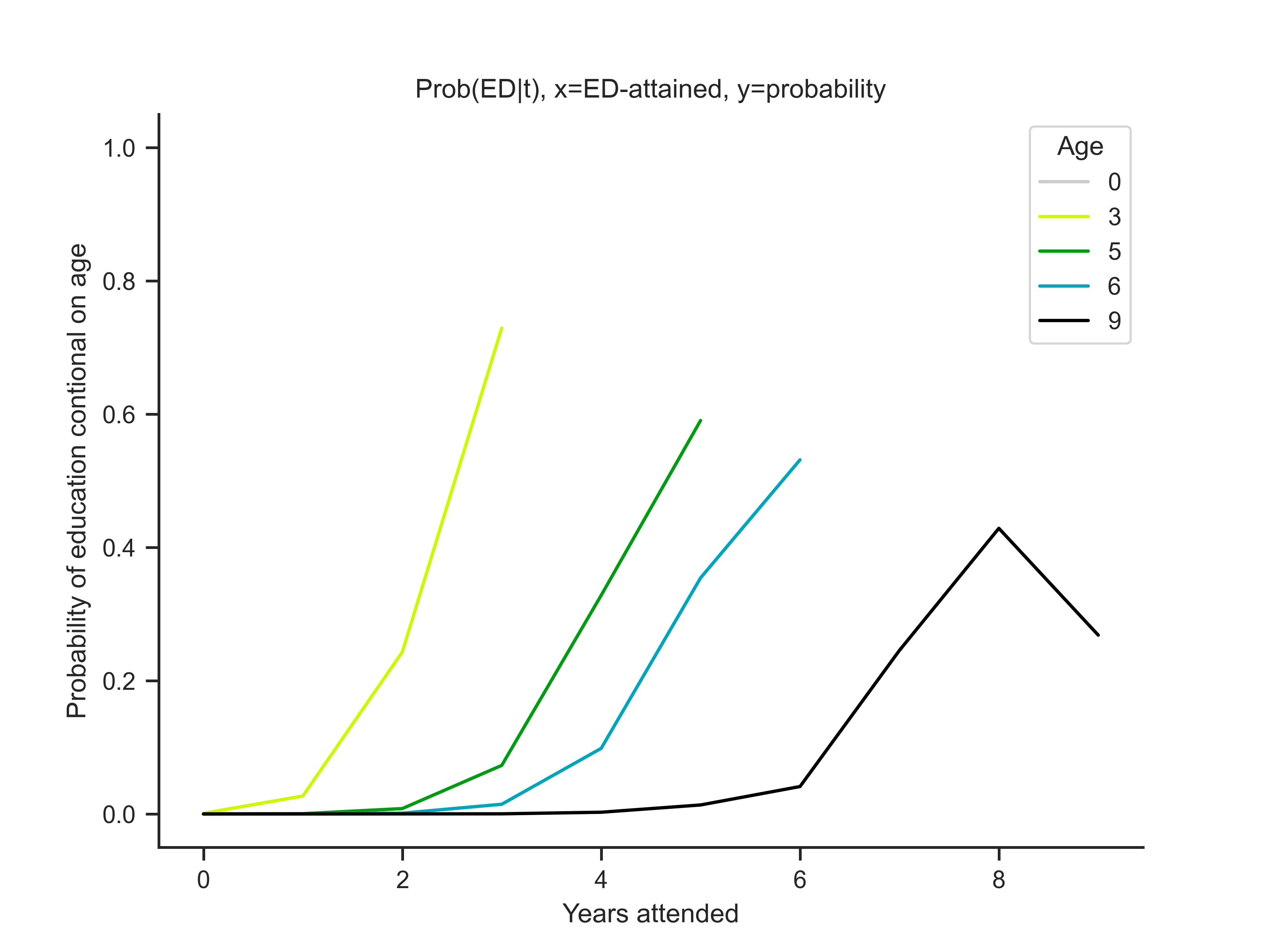
Now we will simulate the probabilities based on our simulated data
probs_s = ams.solution()[1]
prob_sim = np.zeros((age_max,age_max))
prob_sim[0,0] = 1 # Everybody is the same in the begining

for age in range(1,age_max):
    for edu in range(age):
        prob_mass = prob_sim[age-1,edu] # Mass of students in age 0 and with edu 1
        prob_s_age_edu = probs_s[age-1,edu] # P(L = 0 | t = t-1, d = d)
        if np.isnan(prob_s_age_edu):    # Maybe is not possible, but I defined as nan in the model solution
                prob_s_age_edu = 0
        else:
            pass
        prob_sim[age,edu]   = prob_sim[age,edu] + (1-prob_s_age_edu)*prob_mass + \
                              ((1 - ams.prob_progress(edu))*prob_s_age_edu)*prob_mass      # Adding the 0 to the teachers proportion multiplied by the conditional prob to leisure
        prob_sim[age,edu+1] = prob_sim[age,edu+1] + (ams.prob_progress(edu)*prob_s_age_edu)*prob_mass # Same as (214) but now with prob to work
Use a function to calculate discrete probabilities
prob_sim = ams.discrete_probs()
print(prob_sim)
[[1.00000000e+00 0.00000000e+00 0.00000000e+00 0.00000000e+00
  0.00000000e+00 0.00000000e+00 0.00000000e+00 0.00000000e+00
  0.00000000e+00 0.00000000e+00]
 [1.00000066e-01 8.99999934e-01 0.00000000e+00 0.00000000e+00
  0.00000000e+00 0.00000000e+00 0.00000000e+00 0.00000000e+00
  0.00000000e+00 0.00000000e+00]
 [1.00001110e-02 1.80000102e-01 8.09999787e-01 0.00000000e+00
  0.00000000e+00 0.00000000e+00 0.00000000e+00 0.00000000e+00
  0.00000000e+00 0.00000000e+00]
 [1.00019368e-03 2.70004262e-02 2.42999903e-01 7.28999477e-01
  0.00000000e+00 0.00000000e+00 0.00000000e+00 0.00000000e+00
  0.00000000e+00 0.00000000e+00]
 [1.00354846e-04 3.60126474e-03 4.86006713e-02 2.91598849e-01
  6.56098860e-01 0.00000000e+00 0.00000000e+00 0.00000000e+00
  0.00000000e+00 0.00000000e+00]
 [1.04090611e-05 4.53938035e-04 8.10392099e-03 7.28986030e-02
  3.28046228e-01 5.90486900e-01 0.00000000e+00 0.00000000e+00
  0.00000000e+00 0.00000000e+00]
 [1.82958733e-06 5.95118222e-05 1.24075146e-03 1.45804498e-02
  9.84079051e-02 3.54278094e-01 5.31431458e-01 0.00000000e+00
  0.00000000e+00 0.00000000e+00]
 [7.46853746e-07 1.96765498e-05 2.09304680e-04 2.68436462e-03
  2.29358896e-02 1.23945793e-01 3.71941004e-01 4.78263221e-01
  0.00000000e+00 0.00000000e+00]
 [5.24250772e-07 1.29009241e-05 1.11497593e-04 5.71018664e-04
  5.68416388e-03 3.25452241e-02 1.48419947e-01 4.54058688e-01
  3.58596035e-01 0.00000000e+00]
 [4.60830022e-07 1.11206781e-05 1.01415775e-04 2.04580307e-04
  2.59056039e-03 1.35006688e-02 4.11551927e-02 2.45432603e-01
  4.28644222e-01 2.68359176e-01]]
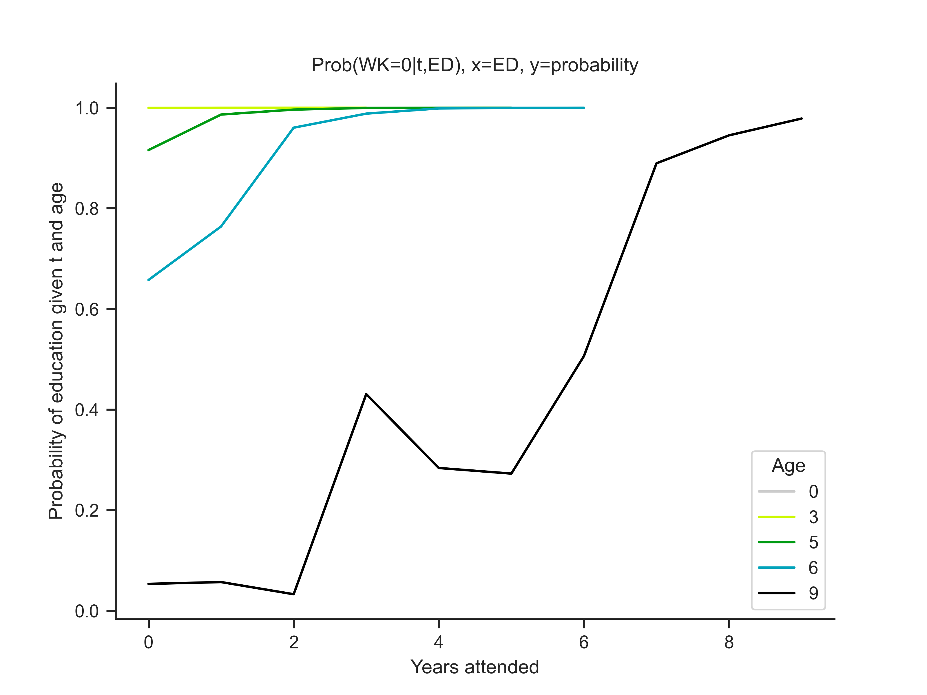
Now we will plot the simulation results
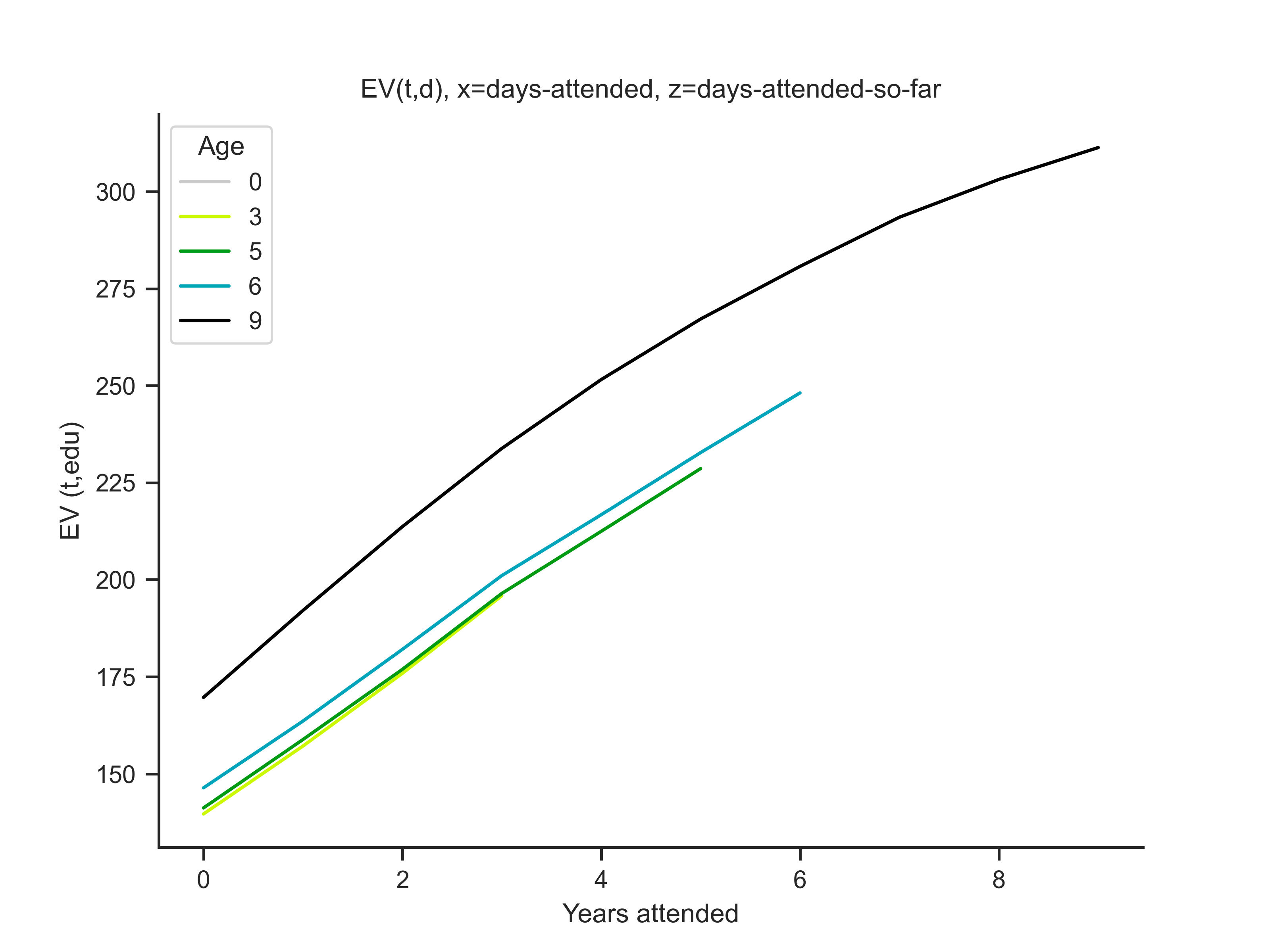
ams.t_graphs()


