Authoring

1 Colors

• Red
• Green
• Blue

2 Shapes

• Square
• Circle
• Triangle

3 Textures

• Smooth
• Bumpy
• Fuzzy

4 Equations

Einstein’s theory of special relatively that expresses the equivalence of mass and energy:

E = mc^{2}

4.1 Bibliography

Knuth says always be literate [@canavire-bacarreza_unintended_2018].

1 + 1

2

4.2 References

5 Cross references

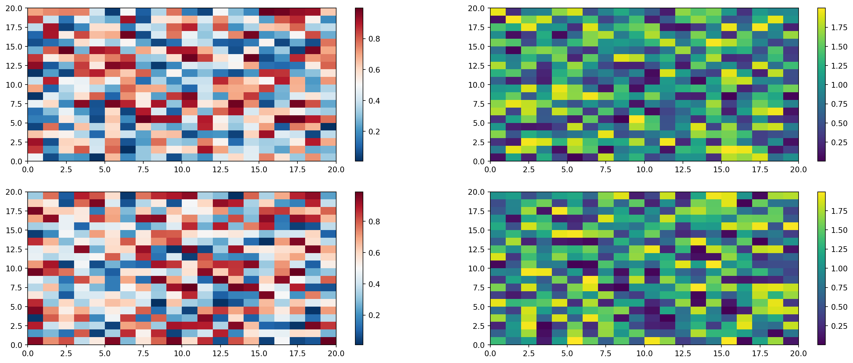
See Figure 1 in Section 5.1 for a demonstration of a simple plot.

See Equation 1 to better understand standard deviation.

5.1 Plot

import matplotlib.pyplot as plt
plt.plot([1,23,2,4])
plt.show()

Figure 1: Simple Plot

5.2 Equation

s = \sqrt{\frac{1}{N-1} \sum_{i=1}^N (x_i - \overline{x})^2} \tag{1}

6 Callout

Note

Note that there are five types of callouts, including: note, tip, warning, caution, and important.

Tip

Note that there are five types of callouts, including: note, tip, warning, caution, and important.

Warning

Note that there are five types of callouts, including: note, tip, warning, caution, and important.

Caution

Note that there are five types of callouts, including: note, tip, warning, caution, and important.

Important

Note that there are five types of callouts, including: note, tip, warning, caution, and important.

7 Article layout

7.1 Placing Colorbars

Colorbars indicate the quantitative extent of image data. Placing in a figure is non-trivial because room needs to be made for them. The simplest case is just attaching a colorbar to each axes:¹.

¹ See the Matplotlib Gallery to explore colorbars further

import matplotlib.pyplot as plt
import numpy as np

fig, axs = plt.subplots(2, 2)
fig.set_size_inches(20, 8)
cmaps = ['RdBu_r', 'viridis']
for col in range(2):
    for row in range(2):
        ax = axs[row, col]
        pcm = ax.pcolormesh(
          np.random.random((20, 20)) * (col + 1),
          cmap=cmaps[col]
        )
        fig.colorbar(pcm, ax=ax)
plt.show()